Factor analytic and reduced rank models in sommer

The sommer package was developed to provide R users with a flexible univariate and multivariate linear mixed-model solver. Multi-environment trial (MET) analyses often need a genetic covariance structure among environments. A fully unstructured covariance (usm()) captures every pairwise environment relationship but requires $q(q+1)/2-1$ parameters for $q$ environments, which quickly becomes difficult to estimate reliably as the number of environments grows. Factor-analytic (FA) and reduced-rank (RR) models approximate that same covariance with far fewer parameters by assuming that genotype-by-environment interaction is driven by a small number of latent factors.

This vignette focuses on the fam() and rrm() covariance-shaping factors used inside vsm(), and on the loadings_mmes()/scores_mmes() helper functions used to extract and visualize their fitted quantities.

SECTION 1: Theory

Why reduce the cross-environment covariance
The factor-analytic (FA) model
The reduced-rank (RR) model
Choosing k and comparing to other structures

SECTION 2: Fitting factor-analytic and reduced-rank models

Data
Factor-analytic model with fam()
Reduced-rank model with rrm()
Comparing FA and RR

SECTION 3: Extracting loadings, scores, and diagnostic plots

Loadings and specific variances
Genotype scores
Why and how to rotate loadings and scores
Percentage of variance explained
Loadings plot
Genotype scores plot
Latent regression plots
Heatmap of the fitted genetic correlation matrix

SECTION 1: Theory

1) Why reduce the cross-environment covariance

Let $q$ be the number of environments and $G$ the $q\times q$ genetic covariance matrix among them. An unstructured model estimates every variance and covariance directly, $q(q+1)/2-1$ working parameters after removing the single overall scale owned by vsm(). As $q$ grows, this saturated model becomes weakly identified relative to the available genotype replication, and its estimates become unstable. Diagonal (dsm()) and compound-symmetry (csm()) models are far more parsimonious but assume, respectively, no genetic correlation among environments or one common correlation everywhere. Factor-analytic and reduced-rank models sit between these extremes: they estimate genuine environment-specific covariance patterns while controlling the number of parameters through a rank $k \ll q$ .

2) The factor-analytic (FA) model

The FA model represents the environment covariance shape as

$K = \Lambda\Lambda^{\mathsf T} + \Psi,$

where $\Lambda$ is a $q\times k$ loading matrix and $\Psi$ is a diagonal matrix of environment-specific variances. Each environment’s genetic variance is split into a part explained by the $k$ common latent factors ( $\Lambda\Lambda^{\mathsf T}$ ) and a part unique to that environment ( $\Psi$ ). vsm() still owns the single overall variance scale, so fam(x, k) reports a normalized shape with $K_{11}=1$ ; the number of estimated working parameters for $k$ factors and $q$ environments is

$kq-\frac{k(k-1)}{2} + (q-1),$

the first term for the (rotationally-constrained, lower-triangular) loadings and the second for the environment-specific variance ratios.

3) The reduced-rank (RR) model

The RR model uses the same loading structure but fixes the environment-specific remainder to be homogeneous:

$K = \Lambda\Lambda^{\mathsf T} + I.$

rrm(x, k) therefore has

$kq-\frac{k(k-1)}{2}$

working parameters: exactly $q-1$ fewer than fam(x, k), because it does not estimate separate environment-specific variances. RR is a restricted (nested) special case of FA in which every environment is assumed to have the same residual/specific variance after accounting for the $k$ common factors. It is useful when there is not enough replication to support $q$ separate specific variances, or as a more parsimonious first approximation before fitting the full FA model.

4) Choosing k and comparing to other structures

Increasing $k$ moves the model continuously from compound symmetry-like behavior ( $k=0$ , not directly supported, but conceptually the limit) toward the saturated unstructured model ( $k=q-1$ ). In practice $k$ is chosen small enough to remain identifiable and interpretable (often 1-3 factors), and increased only if it meaningfully improves the likelihood. Because RR is nested inside FA with the same $k$ , anova.mmes() can be used to test whether the extra $q-1$ FA specific-variance parameters are supported by the data.

SECTION 2: Fitting factor-analytic and reduced-rank models

1) Data

We use the DT_h2 multi-environment potato yield dataset, which has 15 environments (Env, combining location and year) and 41 genotypes (Name).

library(sommer)

## Loading required package: Matrix

## Loading required package: MASS

## Loading required package: crayon

## Loading required package: enhancer

data(DT_h2, package="enhancer")
DT <- DT_h2
DT <- DT[with(DT, order(Env)), ]
length(unique(DT$Env))

## [1] 15

length(unique(DT$Name))

## [1] 41

head(DT)

##          Name     Env Loc Year     Block  y
## 67   MSL007-B CA.2011  CA 2011 CA.2011.2  5
## 105  MSL007-B CA.2011  CA 2011 CA.2011.1  6
## 308  MSK061-4 CA.2011  CA 2011 CA.2011.2  9
## 393  MSK061-4 CA.2011  CA 2011 CA.2011.1 10
## 469 MSR169-8Y CA.2011  CA 2011 CA.2011.1 11
## 471     NY148 CA.2011  CA 2011 CA.2011.1 11

2) Factor-analytic model with `fam()`

fitFA <- mmes(y ~ Env,
              random = ~ vsm(fam(Env, 2), ism(Name)),
              rcov = ~ units,
              nIters = 150, verbose = FALSE,
              data = DT)

## Solver selected: ldlt

summary(fitFA)$varcomp

##                           term                  parameter      estimate
## 1  vsm(fam(Env, 2), ism(Name))        loading[CA.2011,F1]  3.0045084356
## 2  vsm(fam(Env, 2), ism(Name))        loading[CA.2012,F1]  1.5054509348
## 3  vsm(fam(Env, 2), ism(Name))        loading[CA.2013,F1]  1.9757366454
## 4  vsm(fam(Env, 2), ism(Name))        loading[FL.2011,F1]  0.4331622704
## 5  vsm(fam(Env, 2), ism(Name))        loading[FL.2012,F1]  0.1758303920
## 6  vsm(fam(Env, 2), ism(Name))        loading[FL.2013,F1]  0.9721547458
## 7  vsm(fam(Env, 2), ism(Name))        loading[MI.2011,F1]  2.1361012301
## 8  vsm(fam(Env, 2), ism(Name))        loading[MI.2012,F1]  1.4410047879
## 9  vsm(fam(Env, 2), ism(Name))        loading[MI.2013,F1]  2.6984101433
## 10 vsm(fam(Env, 2), ism(Name))        loading[MO.2011,F1]  0.8359231526
## 11 vsm(fam(Env, 2), ism(Name))        loading[MO.2012,F1]  2.2995702105
## 12 vsm(fam(Env, 2), ism(Name))        loading[MO.2013,F1]  1.1781633001
## 13 vsm(fam(Env, 2), ism(Name))        loading[NY.2011,F1]  0.9770518156
## 14 vsm(fam(Env, 2), ism(Name))        loading[NY.2012,F1]  1.3694317830
## 15 vsm(fam(Env, 2), ism(Name))        loading[NY.2013,F1]  0.8890638690
## 16 vsm(fam(Env, 2), ism(Name))        loading[CA.2012,F2]  0.1740475784
## 17 vsm(fam(Env, 2), ism(Name))        loading[CA.2013,F2] -0.5743633396
## 18 vsm(fam(Env, 2), ism(Name))        loading[FL.2011,F2]  1.1951822665
## 19 vsm(fam(Env, 2), ism(Name))        loading[FL.2012,F2]  0.5530367309
## 20 vsm(fam(Env, 2), ism(Name))        loading[FL.2013,F2]  0.1133759961
## 21 vsm(fam(Env, 2), ism(Name))        loading[MI.2011,F2]  1.1599714301
## 22 vsm(fam(Env, 2), ism(Name))        loading[MI.2012,F2]  0.8073883855
## 23 vsm(fam(Env, 2), ism(Name))        loading[MI.2013,F2]  0.9404496750
## 24 vsm(fam(Env, 2), ism(Name))        loading[MO.2011,F2] -0.2444912443
## 25 vsm(fam(Env, 2), ism(Name))        loading[MO.2012,F2]  1.4828667961
## 26 vsm(fam(Env, 2), ism(Name))        loading[MO.2013,F2]  0.6420156516
## 27 vsm(fam(Env, 2), ism(Name))        loading[NY.2011,F2]  2.0650340675
## 28 vsm(fam(Env, 2), ism(Name))        loading[NY.2012,F2]  0.4525037894
## 29 vsm(fam(Env, 2), ism(Name))        loading[NY.2013,F2]  2.8089358980
## 30 vsm(fam(Env, 2), ism(Name)) specific_variance[CA.2011]  6.6631873764
## 31 vsm(fam(Env, 2), ism(Name)) specific_variance[CA.2012]  3.0478110978
## 32 vsm(fam(Env, 2), ism(Name)) specific_variance[CA.2013]  3.6144815675
## 33 vsm(fam(Env, 2), ism(Name)) specific_variance[FL.2011]  0.0512286379
## 34 vsm(fam(Env, 2), ism(Name)) specific_variance[FL.2012]  0.0001680773
## 35 vsm(fam(Env, 2), ism(Name)) specific_variance[FL.2013]  0.0001680737
## 36 vsm(fam(Env, 2), ism(Name)) specific_variance[MI.2011]  3.0532627432
## 37 vsm(fam(Env, 2), ism(Name)) specific_variance[MI.2012]  2.3171167401
## 38 vsm(fam(Env, 2), ism(Name)) specific_variance[MI.2013] 11.2699250853
## 39 vsm(fam(Env, 2), ism(Name)) specific_variance[MO.2011]  0.0002077543
## 40 vsm(fam(Env, 2), ism(Name)) specific_variance[MO.2012]  9.0141847049
## 41 vsm(fam(Env, 2), ism(Name)) specific_variance[MO.2013]  0.0270746727
## 42 vsm(fam(Env, 2), ism(Name)) specific_variance[NY.2011]  0.0004270813
## 43 vsm(fam(Env, 2), ism(Name)) specific_variance[NY.2012]  0.0003026702
## 44 vsm(fam(Env, 2), ism(Name)) specific_variance[NY.2013]  0.3806383153
## 45             vsm(ism(units))                     sigma2  3.9686833132
##     StdError        Zratio
## 1  0.8219473  3.6553538821
## 2  0.4635658  3.2475452968
## 3  0.5735737  3.4446079914
## 4  0.5187481  0.8350147377
## 5  0.3264808  0.5385627535
## 6  0.3677212  2.6437276760
## 7  0.7775142  2.7473470422
## 8  0.4946927  2.9129289140
## 9  0.9133684  2.9543501769
## 10 0.3919781  2.1325763161
## 11 0.8824041  2.6060285029
## 12 0.3731590  3.1572689038
## 13 0.7889468  1.2384254792
## 14 0.3416073  4.0087897593
## 15 0.9713599  0.9152775143
## 16 0.6427593  0.2707819056
## 17 0.8188173 -0.7014547995
## 18 0.4728535  2.5275950871
## 19 0.2964332  1.8656368341
## 20 0.5020510  0.2258256480
## 21 0.8156430  1.4221558099
## 22 0.5440140  1.4841315594
## 23 1.1341122  0.8292386742
## 24 0.4911352 -0.4978084314
## 25 1.0037695  1.4772981197
## 26 0.4671950  1.3741921730
## 27 0.5968049  3.4601495332
## 28 0.4763993  0.9498413799
## 29 0.6534006  4.2989489159
## 30 3.4894220  1.9095389899
## 31 1.3316499  2.2887480420
## 32 1.8766711  1.9260069269
## 33 0.7824268  0.0654740311
## 34 0.5338380  0.0003148471
## 35 0.7542317  0.0002228409
## 36 2.0092531  1.5196008841
## 37 1.1006809  2.1051666478
## 38 3.8942734  2.8939737666
## 39 0.9372746  0.0002216578
## 40 3.2885630  2.7410709878
## 41 0.5877688  0.0460634726
## 42 1.2771970  0.0003343895
## 43 0.5765803  0.0005249403
## 44 2.0168517  0.1887289591
## 45 0.2652345 14.9629249364

3) Reduced-rank model with `rrm()`

fitRR <- mmes(y ~ Env,
              random = ~ vsm(rrm(Env, 2), ism(Name)),
              rcov = ~ units,
              nIters = 150, verbose = FALSE,
              data = DT)

## Solver selected: ldlt

summary(fitRR)$varcomp

##                           term                parameter    estimate  StdError
## 1  vsm(rrm(Env, 2), ism(Name))      loading[CA.2011,F1]  3.38526375 0.5729437
## 2  vsm(rrm(Env, 2), ism(Name))      loading[CA.2012,F1]  1.50570995 0.3886297
## 3  vsm(rrm(Env, 2), ism(Name))      loading[CA.2013,F1]  1.74217569 0.4967484
## 4  vsm(rrm(Env, 2), ism(Name))      loading[FL.2011,F1]  0.59368649 0.5455841
## 5  vsm(rrm(Env, 2), ism(Name))      loading[FL.2012,F1]  0.27419127 0.4049720
## 6  vsm(rrm(Env, 2), ism(Name))      loading[FL.2013,F1]  0.72768006 0.5122535
## 7  vsm(rrm(Env, 2), ism(Name))      loading[MI.2011,F1]  2.52921552 0.6449172
## 8  vsm(rrm(Env, 2), ism(Name))      loading[MI.2012,F1]  1.58291410 0.3995450
## 9  vsm(rrm(Env, 2), ism(Name))      loading[MI.2013,F1]  3.60383114 0.6433876
## 10 vsm(rrm(Env, 2), ism(Name))      loading[MO.2011,F1]  0.84221623 0.5666524
## 11 vsm(rrm(Env, 2), ism(Name))      loading[MO.2012,F1]  2.99822451 0.7640730
## 12 vsm(rrm(Env, 2), ism(Name))      loading[MO.2013,F1]  1.25769810 0.4417988
## 13 vsm(rrm(Env, 2), ism(Name))      loading[NY.2011,F1]  1.81822767 0.7629436
## 14 vsm(rrm(Env, 2), ism(Name))      loading[NY.2012,F1]  1.24649603 0.4089558
## 15 vsm(rrm(Env, 2), ism(Name))      loading[NY.2013,F1]  1.60011259 0.4930630
## 16 vsm(rrm(Env, 2), ism(Name))      loading[CA.2012,F2]  0.49341983 0.4620680
## 17 vsm(rrm(Env, 2), ism(Name))      loading[CA.2013,F2] -1.32493948 0.5255037
## 18 vsm(rrm(Env, 2), ism(Name))      loading[FL.2011,F2]  0.74954406 0.5817799
## 19 vsm(rrm(Env, 2), ism(Name))      loading[FL.2012,F2]  0.25399154 0.4658749
## 20 vsm(rrm(Env, 2), ism(Name))      loading[FL.2013,F2]  0.34678933 0.7057476
## 21 vsm(rrm(Env, 2), ism(Name))      loading[MI.2011,F2]  1.13601042 0.5806006
## 22 vsm(rrm(Env, 2), ism(Name))      loading[MI.2012,F2]  0.49138344 0.4247761
## 23 vsm(rrm(Env, 2), ism(Name))      loading[MI.2013,F2] -1.48915669 0.6406997
## 24 vsm(rrm(Env, 2), ism(Name))      loading[MO.2011,F2] -0.04159525 0.6090733
## 25 vsm(rrm(Env, 2), ism(Name))      loading[MO.2012,F2]  2.51130317 0.6658115
## 26 vsm(rrm(Env, 2), ism(Name))      loading[MO.2013,F2] -0.15382312 0.5293342
## 27 vsm(rrm(Env, 2), ism(Name))      loading[NY.2011,F2]  1.67277032 0.6557797
## 28 vsm(rrm(Env, 2), ism(Name))      loading[NY.2012,F2]  0.31199889 0.4702273
## 29 vsm(rrm(Env, 2), ism(Name))      loading[NY.2013,F2]  1.30639248 0.4805937
## 30 vsm(rrm(Env, 2), ism(Name)) common_specific_variance  1.76752303 0.3366857
## 31             vsm(ism(units))                   sigma2  4.24061722 0.2923704
##         Zratio
## 1   5.90854526
## 2   3.87440791
## 3   3.50715902
## 4   1.08816686
## 5   0.67706236
## 6   1.42054667
## 7   3.92176773
## 8   3.96179158
## 9   5.60133762
## 10  1.48630130
## 11  3.92400263
## 12  2.84676646
## 13  2.38317441
## 14  3.04799728
## 15  3.24524986
## 16  1.06785101
## 17 -2.52127518
## 18  1.28836361
## 19  0.54519253
## 20  0.49137872
## 21  1.95661246
## 22  1.15680576
## 23 -2.32426631
## 24 -0.06829268
## 25  3.77179305
## 26 -0.29059736
## 27  2.55081145
## 28  0.66350652
## 29  2.71828859
## 30  5.24977100
## 31 14.50426198

4) Comparing FA and RR

Because rrm(Env, 2) is nested inside fam(Env, 2) (both use rank 2, but RR fixes the specific variances to be equal), we can compare them with a likelihood ratio test:

c(AIC_FA = fitFA$AIC, AIC_RR = fitRR$AIC)

##     AIC_FA     AIC_RR 
## -144.60423  -72.58435

anova.mmes(fitFA, fitRR)

## Likelihood ratio test for mixed models
## ==============================================================
##      Df        AIC        BIC    loLik    Chisq ChiDf                  PrChisq
## mod1 60 -144.60423 -73.042386 87.30211                                        
## mod2 46  -72.58435  -1.022506 51.29217 72.01988    14 8.29394571269746e-10 ***
## ==============================================================
## Signif. codes:  0 '***' 0.001 '**' 0.01 '*' 0.05 '.' 0.1 ' ' 1

##      Df        AIC        BIC    loLik    Chisq ChiDf                  PrChisq
## mod1 60 -144.60423 -73.042386 87.30211                                        
## mod2 46  -72.58435  -1.022506 51.29217 72.01988    14 8.29394571269746e-10 ***

A lower AIC/BIC and a significant likelihood ratio test favor the less restrictive FA model whenever the data support heterogeneous environment-specific variances.

SECTION 3: Extracting loadings, scores, and diagnostic plots

1) Loadings and specific variances

loadings_mmes() reconstructs the fitted loadings and specific variances. Here we request varianceScale = FALSE explicitly to obtain the normalized loadings $\Lambda$ and specific variances $\Psi$ , so that $\sigma^2(\Lambda\Lambda^{\mathsf T}+\Psi)$ reproduces the fitted covariance matrix. The default rotation = TRUE returns rotated loadings; rotation does not change this covariance.

faInfo <- loadings_mmes(fitFA, varianceScale = FALSE, rotation = TRUE)
round(faInfo$loadings, 3)

##            F1     F2
## CA.2011 0.673  0.350
## CA.2012 0.358  0.136
## CA.2013 0.376  0.359
## FL.2011 0.236 -0.217
## FL.2012 0.104 -0.103
## FL.2013 0.231  0.088
## MI.2011 0.614 -0.011
## MI.2012 0.417 -0.013
## MI.2013 0.714  0.103
## MO.2011 0.159  0.152
## MO.2012 0.688 -0.065
## MO.2013 0.339 -0.007
## NY.2011 0.459 -0.349
## NY.2012 0.359  0.058
## NY.2013 0.526 -0.526

round(faInfo$specific, 3)

## CA.2011 CA.2012 CA.2013 FL.2011 FL.2012 FL.2013 MI.2011 MI.2012 MI.2013 MO.2011 
##   0.425   0.194   0.230   0.003   0.000   0.000   0.195   0.148   0.718   0.000 
## MO.2012 MO.2013 NY.2011 NY.2012 NY.2013 
##   0.575   0.002   0.000   0.000   0.024

faInfo$sigma2

## [1] 15.69026

rrInfo <- loadings_mmes(fitRR, varianceScale = FALSE, rotation = TRUE)
round(rrInfo$specific, 3)

## CA.2011 CA.2012 CA.2013 FL.2011 FL.2012 FL.2013 MI.2011 MI.2012 MI.2013 MO.2011 
##   0.134   0.134   0.134   0.134   0.134   0.134   0.134   0.134   0.134   0.134 
## MO.2012 MO.2013 NY.2011 NY.2012 NY.2013 
##   0.134   0.134   0.134   0.134   0.134

Notice that rrInfo$specific is constant across environments: this is the direct consequence of rrm() fixing a homogeneous specific variance, unlike the heterogeneous values in faInfo$specific.

2) Genotype scores

scores_mmes() predicts each genotype’s position on the $k$ latent factors from its BLUPs, the fitted loadings, and the fitted covariance. We use the default regression method and varianceScale = TRUE: scores are then on the standardized latent-factor scale, with the overall genetic scale absorbed into the corresponding loadings. The term “regression” here describes the score estimator, not a new regression fitted to the plotted points.

faScores <- scores_mmes(fitFA, method = "regression",
                       varianceScale = TRUE, rotation = TRUE)
head(faScores)

##                      F1          F2
## A01143-3C   1.183865871  1.37984105
## AC00206-2W  0.008413789 -0.33761657
## AC01151-5W  0.548584981 -0.09988729
## AC03433-1W -1.025722881 -0.10465079
## AC03452-2W  2.001511977 -0.18606190
## AC05153-1W -1.175685335 -0.37339395

3) Why and how to rotate loadings and scores

The fitted covariance identifies a latent subspace, not a unique set of factor axes. For any orthogonal $k\times k$ matrix $Q$ , with $Q Q^{\mathsf T}=I$ ,

$(\Lambda Q)(\Lambda Q)^{\mathsf T}=\Lambda\Lambda^{\mathsf T}.$

Consequently, many loading matrices describe exactly the same model. The lower-triangular constraints used during fitting identify one parameterization, but its axes depend on the ordering of environments and need not be convenient for interpretation. Rotation at extraction is a change of coordinates, not a refit: it leaves the likelihood, specific variances, genetic covariance, and fitted genotype-by-environment effects unchanged.

Both loadings_mmes() and scores_mmes() accept the logical argument rotation:

rotation = FALSE retains the fitted, lower-triangular loading orientation.
rotation = TRUE (the default) rotates using the right singular vectors of the loading matrix. If $\Lambda=A D V^{\mathsf T}$ is its singular value decomposition, sommer uses $Q=-V$ and returns $\Lambda_* = \Lambda Q$ . The loading columns are then orthogonal, ordered by decreasing squared length. This is an SVD rotation, not a varimax or oblique rotation; no rotation name or custom matrix is accepted by this argument.

The rotated first factor captures the largest share of the common genetic variance; subsequent factors capture decreasing shares. When first-factor loadings have the same sign across environments, that factor can describe broad performance, while later factors describe contrasting responses or crossover interaction. This interpretation is data-dependent: the first factor is not necessarily an overall-performance axis, and later factors are not automatically particular environmental variables.

Always rotate loadings and scores together. Writing $L=\sqrt{\sigma^2}\Lambda$ for the loadings in trait units and $F$ for the genotype-by-factor score matrix, the common genetic prediction is

$\widehat U_{\mathrm{common}} = F L^{\mathsf T}.$

With $L_* = LQ$ and $F_* = FQ$ , this product is unchanged. Mixing rotated scores with unrotated loadings gives incorrect reconstructions and misleading plots. Keep term, method, and varianceScale consistent across extraction calls as well. Here the normalized loadings in faInfo are converted to trait units explicitly to match faScores:

faUnrotated <- loadings_mmes(fitFA, varianceScale = FALSE,
                           rotation = FALSE)
scoresUnrotated <- scores_mmes(fitFA, method = "regression",
                              varianceScale = TRUE, rotation = FALSE)
L <- sqrt(faInfo$sigma2) * faInfo$loadings
LUnrotated <- sqrt(faUnrotated$sigma2) * faUnrotated$loadings
common <- faScores %*% t(L)
commonUnrotated <- scoresUnrotated %*% t(LUnrotated)

stopifnot(
  isTRUE(all.equal(tcrossprod(L), tcrossprod(LUnrotated))),
  isTRUE(all.equal(common, commonUnrotated)),
  isTRUE(all.equal(faInfo$specific, faUnrotated$specific))
)
round(crossprod(L), 3)

##        F1     F2
## F1 49.137  0.000
## F2  0.000 12.159

The same arguments and reasoning apply to fitRR. For one factor there is no multi-axis rotation, only a possible sign change. A factor’s sign is arbitrary: reversing both a loading column and its score column changes neither the covariance nor the common predictions. Thus a negative score is not intrinsically “poor performance”; interpret it together with the loadings. Across separate fits, axes can also swap or become unstable when singular values are nearly equal, so raw score signs and labels should not be compared without aligning the axes.

This extraction argument is distinct from vsm(..., Gu = Gu, rotation = TRUE), which requests Lee–van der Werf rotation of a relationship term during fitting, not the post-fit orientation of FA/RR factors.

4) Percentage of variance explained

A standard factor-analytic diagnostic is the proportion of total genetic variance attributed to each latent factor:

varPerFactor <- colSums(faInfo$loadings^2)
totalVar <- sum(faInfo$loadings^2) + sum(faInfo$specific)
propExplained <- varPerFactor / totalVar
round(100 * propExplained, 1)

##   F1   F2 
## 48.8 12.1

These percentages use the normalized loadings and specific variances, so the common overall scale cancels. Their sum is the percentage of total genetic variance explained by the common factors, not necessarily 100%. Rotation redistributes variance between factors but preserves that sum. Under the default SVD rotation, factors are ordered by decreasing contribution; the percentages refer to variance across environments, not phenotypic variance or genotype-specific prediction accuracy.

5) Loadings plot

Plotting the loadings by environment shows which environments are most associated with each latent factor.

barplot(t(faInfo$loadings), beside = TRUE,
        col = c("steelblue4", "tomato"),
        las = 2, cex.names = 0.7,
        ylab = "Loading",
        main = "Factor-analytic loadings by environment")
legend("topright", legend = colnames(faInfo$loadings),
       fill = c("steelblue4", "tomato"), bty = "n")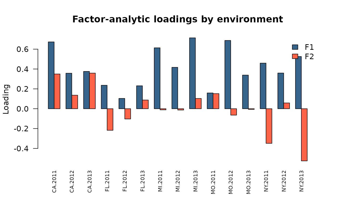

6) Genotype scores plot

This is a plot of genotype scores only, rather than a biplot containing both genotype scores and environment loadings. Genotypes close together have similar common-factor responses, although their environment-specific effects may differ. The signs and directions must be read alongside the loading plot.

plot(faScores[,2] ~ faScores[,1],
     xlab = "Factor 1 score", ylab = "Factor 2 score",
     main = "Genotype scores")
text(faScores[,2] ~ faScores[,1], labels = rownames(faScores),
     cex = 0.6, pos = 1)
abline(h = 0, v = 0, lty = 3)

7) Latent regression plots

In the FA literature, a latent regression plot displays genotype performance against an environmental coordinate estimated by the model: a factor loading. Unlike regression on measured rainfall or temperature, the horizontal coordinate is latent and learned from the genetic covariance. Each genotype has its own regression slope, given by its factor score. Such plots help distinguish broad adaptation from sensitivity to the environmental contrasts captured by a factor; see Smith and Cullis (2018) for FA-based selection tools and interpretation of performance and stability.

For genotype $g$ in environment $e$ , the genetic effect is decomposed as

$\widehat u_{ge} = \sum_{j=1}^k \widehat f_{gj} L_{ej} + \widehat\delta_{ge},$

where $\widehat\delta_{ge}$ is the predicted environment-specific remainder. In a one-factor model the common response is the straight line $\widehat f_{g1} L_{e1}$ through the origin. With multiple factors, plotting the full genetic effect against only one loading also includes contributions from the other factors. To isolate factor $j$ , subtract those contributions first:

$\widehat u_{ge}^{(j)} = \widehat u_{ge} - \sum_{h\ne j}\widehat f_{gh} L_{eh} = \widehat f_{gj} L_{ej} + \widehat\delta_{ge}.$

The following base-R plots show these adjusted genetic BLUPs as points and the common-factor response as a line. We select four genotypes spanning the rotated first-factor scores to keep the display readable. Their selection is illustrative, not a ranking rule.

U <- fitFA$uList[[faInfo$term]]
U <- U[rownames(faScores), rownames(L), drop = FALSE]
specificBLUP <- U - common
scoreOrder <- order(faScores[, 1])
selected <- scoreOrder[unique(round(seq(1, length(scoreOrder),
                                       length.out = 4)))]
genotypeColors <- c("steelblue4", "tomato3", "darkgreen", "goldenrod3")

local({
  oldPar <- par(mfrow = c(1, ncol(L)), mar = c(4.5, 4.5, 3, 1))
  on.exit(par(oldPar))
  for (factorIndex in seq_len(ncol(L))) {
    loading <- L[, factorIndex]
    factorResponse <- outer(faScores[selected, factorIndex], loading)
    adjusted <- factorResponse + specificBLUP[selected, , drop = FALSE]
    plot(range(loading), range(c(adjusted, factorResponse, 0)),
         type = "n", xlab = paste("Environment loading:", colnames(L)[factorIndex]),
         ylab = "Adjusted genetic effect", main = paste("Latent regression", factorIndex))
    abline(h = 0, v = 0, lty = 3, col = "grey70")
    for (genotypeIndex in seq_along(selected)) {
      points(loading, adjusted[genotypeIndex, ], pch = 16,
             col = genotypeColors[genotypeIndex])
      abline(a = 0, b = faScores[selected[genotypeIndex], factorIndex],
             col = genotypeColors[genotypeIndex], lwd = 2)
    }
    legend("topleft", legend = rownames(faScores)[selected],
           col = genotypeColors[seq_along(selected)], pch = 16, lty = 1,
           cex = 0.7, bty = "n")
  }
})

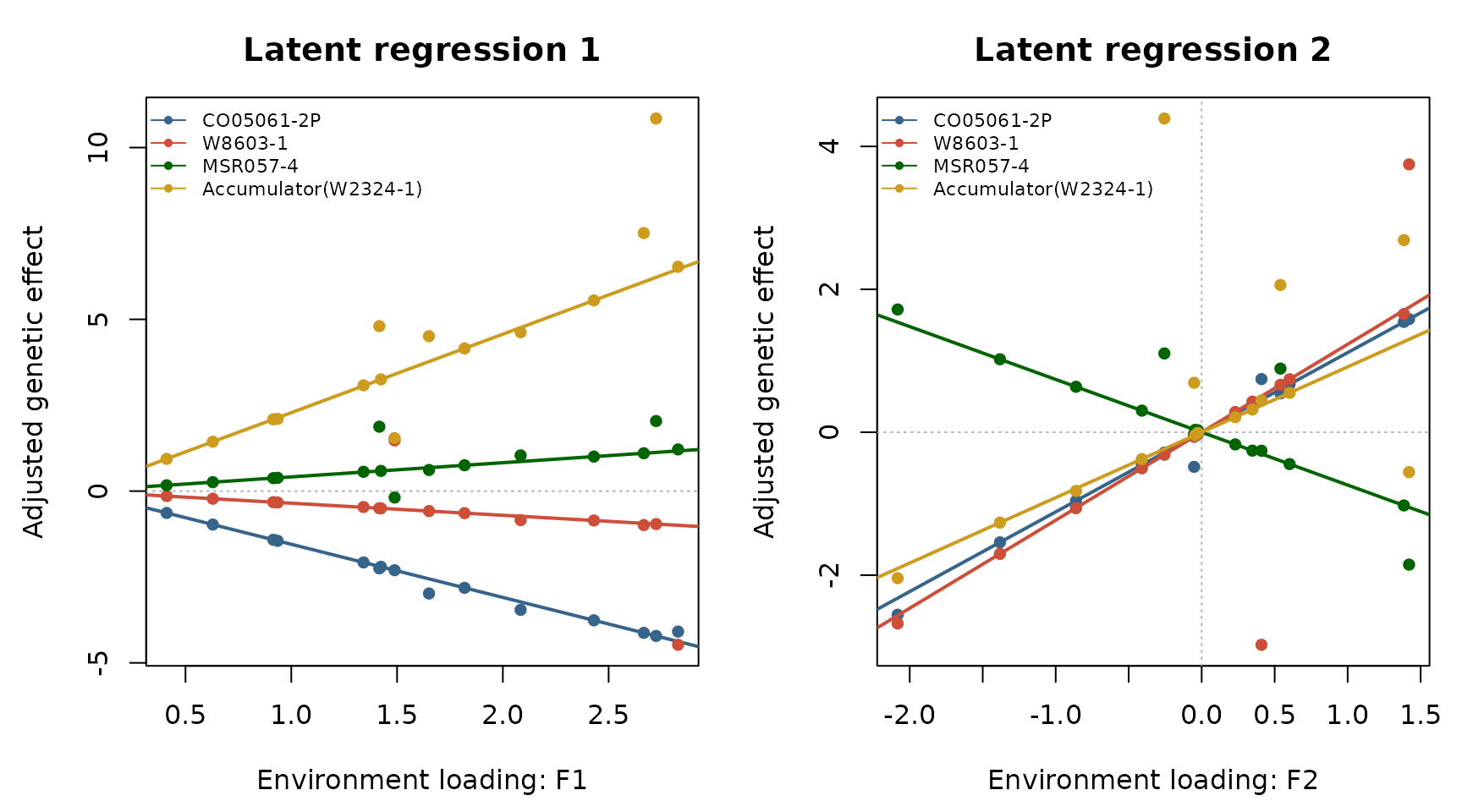
Each point represents an environment, located at its loading on that factor. A steep slope indicates a strong response to that latent environmental contrast; a nearly flat slope indicates little response along that axis. Opposite slopes indicate contrasting responses. Points away from a genotype’s line reflect the environment-specific remainder after removing the other factors, not raw observation residuals. The lines use model-derived scores; they are not ordinary least-squares regressions fitted to these points.

These are plots of genetic deviations, not absolute yield: the fixed environment effects are omitted, so all common-factor lines pass through zero and their crossings alone do not establish differences in total yield. For selection, consider the full predicted genetic effects (or predictions including fixed effects), all retained factors, specific effects, and prediction uncertainty. The points are shrunken BLUPs, and uncertainty in both loadings and scores is not shown. The default regression scores and Bartlett scores need not give the same slopes; use one method consistently. To draw analogous RR plots, extract the RR loadings and scores with the same rotation and scale choices and use the RR term’s BLUP matrix.

8) Heatmap of the fitted genetic correlation matrix

The normalized loadings and specific variances returned by loadings_mmes() can be combined directly into the fitted genetic covariance, and then converted to a correlation matrix for visualization.

Sigma <- faInfo$sigma2 * (
  faInfo$loadings %*% t(faInfo$loadings) + diag(faInfo$specific)
)
corMat <- cov2cor(Sigma)
stopifnot(isTRUE(all.equal(unname(Sigma),
                          unname(fitFA$theta[[faInfo$term]]))))
heatmap(corMat, symm = TRUE,
        main = "Fitted genetic correlation among environments")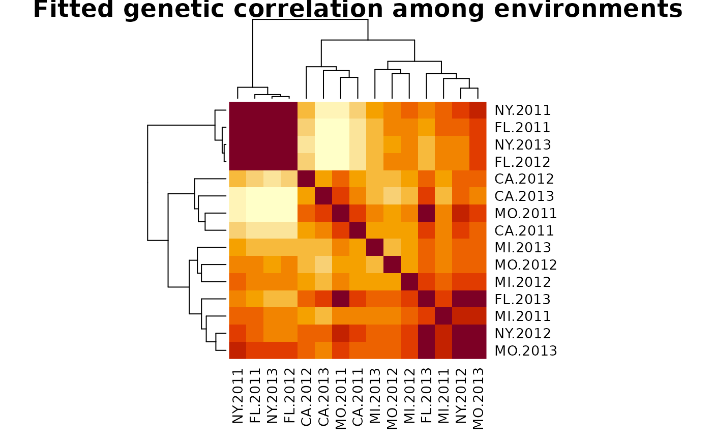

Environments with a strong positive fitted correlation cluster together in the heatmap, while environments explained by different latent factors, or with a large specific variance, appear less correlated with the rest.

Literature

Covarrubias-Pazaran G. 2016. Genome assisted prediction of quantitative traits using the R package sommer. PLoS ONE 11(6):1-15.

Smith AB, Cullis BR, Thompson R. 2001. Analyzing variety by environment data using multiplicative mixed models and expectations of trials. Biometrics 57(4).

Thompson R, Cullis B, Smith A, Gilmour A. 2003. A sparse implementation of the average information algorithm for factor analytic and reduced rank variance models. Australian & New Zealand Journal of Statistics 45(4).

Smith AB, Cullis BR. 2018. Plant breeding selection tools built on factor analytic mixed models for multi-environment trial data. Euphytica 214:143. https://doi.org/10.1007/s10681-018-2220-5.

Gilmour AR, Thompson R, Cullis BR. 1995. Average Information REML: An efficient algorithm for variance parameter estimation in linear mixed models. Biometrics 51:1440-1450.

Giovanny Covarrubias-Pazaran

2026-10-06

SECTION 1: Theory

1) Why reduce the cross-environment covariance

2) The factor-analytic (FA) model

3) The reduced-rank (RR) model

4) Choosing k and comparing to other structures

SECTION 2: Fitting factor-analytic and reduced-rank models

1) Data

2) Factor-analytic model with `fam()`

3) Reduced-rank model with `rrm()`

4) Comparing FA and RR

SECTION 3: Extracting loadings, scores, and diagnostic plots

1) Loadings and specific variances

2) Genotype scores

3) Why and how to rotate loadings and scores

4) Percentage of variance explained

5) Loadings plot

6) Genotype scores plot

7) Latent regression plots

8) Heatmap of the fitted genetic correlation matrix

Literature

Factor analytic and reduced rank models in sommer

Giovanny Covarrubias-Pazaran

2026-10-06

SECTION 1: Theory

1) Why reduce the cross-environment covariance

2) The factor-analytic (FA) model

3) The reduced-rank (RR) model

4) Choosing k and comparing to other structures

SECTION 2: Fitting factor-analytic and reduced-rank models

1) Data

2) Factor-analytic model with fam()

3) Reduced-rank model with rrm()

4) Comparing FA and RR

SECTION 3: Extracting loadings, scores, and diagnostic plots

1) Loadings and specific variances

2) Genotype scores

3) Why and how to rotate loadings and scores

4) Percentage of variance explained

5) Loadings plot

6) Genotype scores plot

7) Latent regression plots

8) Heatmap of the fitted genetic correlation matrix

Literature

2) Factor-analytic model with `fam()`

3) Reduced-rank model with `rrm()`